Hypothesis testing for Binomial (A-level Maths)

In the first year of the A-level Maths course you need to be able to carry out a hypothesis test to judge whether a Binomial probability has (probably) changed.
In the second year, hypothesis tests are required (1) to decide whether the mean of a Normal distribution has changed, and (2) to ascertain whether correlation exists in a population.

This tutorial introduces the concept of a hypothesis test and explains how it works with a Binomial probability. You can find the lesson on hypothesis testing for Normal here, and the one on correlation / pmcc here.

You will need to have an understanding of how to calculate probabilities using the Binomial Distribution before this article will make sense to you!

What is hypothesis testing?

The purpose of hypothesis testing

We use hypothesis testing to decide whether it’s likely that something has changed; in the case of a Binomial Distribution the question is whether the probability of success has changed from its historical value.

For example, a company might have made changes to its flexible working policies and want to know whether that has reduced the number of staff calling in sick, or a sports team that has brought in a new coach might want to know whether the team’s win rate has changed as a result.

How it works – basic principle

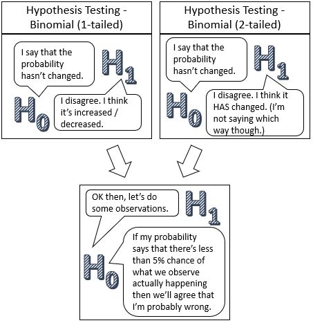
H₀ is the null hypothesis, which is the assertion that the probability of “success” (however that’s defined) hasn’t changed.
In the first example above, the probability of success might be defined as the proportion of workers who call in sick on average each day (yes, calling in sick is classed as “success” in this context!). In the second one it might be the proportion of games that the team has won in under the previous coach, i.e. the historical probability of a win.

H₁ is the alternative hypothesis, which is the assertion that the probability has changed. If the direction of change is specified then it’s a 1-tailed test; if not – effectively H₁ is sitting on the fence and not committing either way – then it’s a 2-tailed test.

We observe the number of successes in a known number of trials and work out what the probability of that (or a more extreme) result would be if the probability hadn’t changed.

If it’s sufficiently unlikely then we reject H₀ and accept that there probably has been a change.

Note: Because it’s all based on a balance of probabilities, you can never make a definitive statement that yes, the value in question HAS changed, only that it’s likely that it’s no longer the same as before. Therefore the question is always whether we reject H₀, not whether we accept H₁.

The significance level

The significance level, α, dictates how demanding the test is. If the significance level is 10%, or α = 0.1, then we’re looking to see whether the probability of the observed result (under the old probability) is less than 0.1. If it is then the result is considered significant and we reject H₀.

If α is 5%, or 0.05, then the probability has to be less than 0.05 for H₀ to be rejected – so you’re less likely to reject H₀ and to agree that the probability has most likely changed.

The significance level is also the probability of incorrectly rejecting H₀. This is because although the observed result may be unlikely, it is still possible under the old probability. At a 5% level of significance, 5% of results would be in the critical region, so it may still be a genuine result under the old probability, just one at the outer edges of what’s normally observed.

Hypothesis testing for Binomial: Carrying out a 1-tailed test

Example

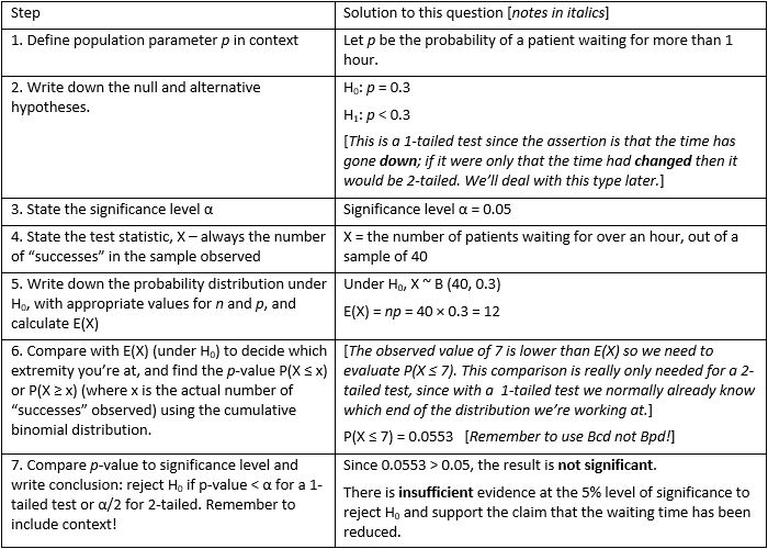
Typically, 3 in 10 patients at a minor injuries unit have to wait more than an hour to be seen. The hospital makes some changes and, out of a subsequent sample of 40 patients, only 7 are found to have waited for more than an hour. The hospital’s management claims that waiting times have been reduced. Test, at the 5% significance level, whether this claim is justified.

Solution

The table below presents a generic writing frame and model solution to the example question side by side, but the text may be too small to display clearly on a mobile screen, so a plain text version is also provided below.

You can get a free printable copy – as well as other useful downloads – if you sign up to my mailing list – see this page.

Writing frame (plain text version)

1. Define population parameter p in context
2. Write down the null and alternative hypotheses.
3. State the significance level α.
4. State the test statistic, X – always the number of “successes” in the sample observed.
5. Write down the probability distribution under H₀, with appropriate values for n and p, and calculate E(X) (the expected, or mean, number of successes in a sample of size n, given by np).
6. Compare with E(X) (under H₀) to decide which extremity you’re at, and find the p-value P(X ≤ x) or P(X ≥ x) (where x is the actual number of “successes” observed) using the cumulative binomial distribution. (This comparison is really only needed for a 2-tailed test, since with a  1-tailed test we normally already know which end of the distribution we’re working at.)
7. Compare p-value to significance level and write conclusion: reject H₀ if p-value < α for a 1-tailed test or α/2 for 2-tailed. Remember to include context!

Solution to example (plain text version)

1. Let p be the probability of a patient waiting for more than 1 hour.
2. H₀: p = 0.3     
   H₁: p < 0.3
   [This is a 1-tailed test since the assertion is that the time has gone down; if it were only that the time had changed then it would be 2-tailed. We’ll deal with this type later.]
3. Significance level α = 0.05
4. X = the number of patients waiting for over an hour, out of a sample of 40.
5. Under H₀, X ~ B (40, 0.3) and E(X) = np = 40 × 0.3 = 12
6. [The observed value of 7 is lower than E(X) so we need to evaluate P(X ≤ 7).]
   P(X ≤ 7) = 0.0553   [Remember to use Bcd not Bpd!]
7. Since 0.0553 > 0.05, the result is not significant. There is insufficient evidence at the 5% level of significance to reject H₀ and support the claim that the waiting time has been reduced.

In other words…

If p is still 0.3 then the probability of 7 or fewer people out of a sample of 40 having to wait more than an hour is 0.0553. This is more likely than the threshold probability of 0.05 dictated by the significance level, so it’s not sufficiently unlikely for us to conclude that p probably has changed and to reject H₀.

If the significance level had been 10% (α = 0.1) then the observed outcome would have had a lower probability than this and so the final part would read:

Since 0.0553 < 0.1, the result is significant.
There is sufficient evidence at the 10% level of significance to reject H₀ and support the claim that the waiting time has been reduced. [Echo the question here!]

However, we mustn’t forget that the significance level of 10% means there’s a 10% probability that the decision to reject H₀ was wrong!

Your turn 1

A school’s records show that 43% of students achieve a Grade 7 or higher in GCSE Maths in a normal year. One year, the assessment system is changed and 17 out of 30 students achieve Grade 7 or above. Test, at the 5% level of significance, the claim that the probability of a student achieving Grade 7 or better has increased.

Work through the writing frame, using the example solution above as a model, then check your answers by clicking on the link below.

Click here for the solution

Finding the critical region (1-tailed test)

The critical region is the range of observed results that would result in H₀ being rejected. The acceptance region is everything that’s not in the critical region.

To find the critical region, you need to identify the value of X where the result changes from not significant to significant. The Classwiz fx-991EX and CW Binomial Distribution functions have a List mode that’s useful for this, as it allows you to calculate several probabilities at the same time.

Going back to Example 1, P(X ≤ 7) = 0.553, which is not significant at the 5% level. But if you calculate the probability for the next value down, P(X ≤ 6), then you’ll find that that’s 0.0238, which is less than 0.05 and so is significant. So the critical region in this case is X ≤ 6, i.e. if the number of patients waiting an hour or longer is 6 or fewer then there is sufficient evidence to reject H₀.

Note: Occasionally you might be asked to use the value that gives a probability closest to the critical value threshold rather than the first one that’s actually in the critical region. If that had been the case for Example 1 then the critical region would have been X ≤ 7 since that has a probability closer to 0.05 than X ≤ 6 does.

Can you identify the critical region for the “Your turn 1” question above?

Click here for the solution

Hypothesis testing for Binomial: Carrying out a 2-tailed test

Example

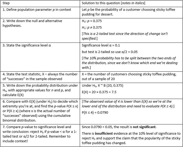
A pub adds whisky to its sticky toffee pudding recipe. The old recipe was chosen by 3 out of every 8 people who had a dessert. After the recipe change, sticky toffee pudding is chosen by 4 people out of the next 20 who have a dessert. Test, at the 10% level, the claim that the popularity of the sticky toffee pudding has changed.

Solution

The only difference here is that H₁ is “hedging its bets” by not specifying whether the popularity of the pudding has increased or decreased, so we have to divide the critical 10% probability between the upper and lower ends of the distribution.

Again, a plain-text version of the table is provided further down the page.

Writing frame (plain text version)

1. Define population parameter p in context
2. Write down the null and alternative hypotheses.
3. State the significance level α and halve it for a 2-tailed test.
4. State the test statistic, X – always the number of “successes” in the sample observed.
5. Write down the probability distribution under H₀, with appropriate values for n and p, and calculate E(X).
6. Compare with E(X) (under H₀) to decide which extremity you’re at, and find the p-value P(X ≤ x) or P(X ≥ x) (where x is the actual number of “successes” observed) using the cumulative binomial distribution.
7. Compare p-value to significance level and write conclusion: reject H₀ if p-value < α for a 1-tailed test or α/2 for 2-tailed. Remember to include context!

Solution to example (plain text version)

1. Let p be the probability of a customer choosing sticky toffee pudding for dessert.
2. H₀: p = 0.375
   H₁: p ≠ 0.375
   [This is a 2-tailed test since the direction of change isn’t specified.]
3. Significance level α = 0.1
   but test is 2-tailed so use α/2 = 0.05
   [The 10% probability has to be split between the two ends of the distribution, since we don’t know which end we’re dealing with.]
4. X = the number of customers choosing sticky toffee pudding, out of a sample of 20.
5. Under H₀, X ~ B (20, 0.375)
   E(X) = 20 × 0.375 = 7.5
6. [The observed value of 4 is lower than E(X) so we know we’re at the lower end of the distribution and need to evaluate P(X ≤ 4).]
   P(X ≤ 4) = 0.0790
7. Since 0.0790 > 0.05, the result is not significant. There is insufficient evidence at the 10% level of significance to reject H₀ and support the claim that the popularity of the sticky toffee pudding has changed.

Your turn 2

32% of students at a particular college achieved grade B or above in A-level Maths. The college changes to a different exam board and 28 out of 60 students achieve B or above. It is claimed that the proportion of students achieving Grade B or above has changed. Test this claim at the 5% significance level.

Work through the writing frame, using the example solution above as a model, then check your answers by clicking on the link below.

Click here for the solution

Finding the critical region (2-tailed test)

For a 2-tailed test, we need a critical region at each end of the distribution. Here’s how to do it for Example 2, keeping the significance level at 10%. Remember, the significance level of 10% had to be split to give 5% at each end of the distribution, so the threshold probability at each end is 0.05.

Starting with the lower end:
P(X ≤ 4) = 0.0790             
[too high so go lower]
P(X ≤ 3) = 0.0271
[this is the first value less than 0.05 so it’s the value we need for the lower end]   

Now the top end: For P(X ≥ x) to be less than 0.05, we need P(X < x) > 0.95
… but of course since it’s a discrete distribution, what we actually need to look up is P(X ≤ (x – 1)) > 0.95

P(X ≤ 10) = 0.9153
[too low so go higher]
P(X ≤ 11) = 0.9657
[this is the first value greater than 0.95 so it’s the value we need for the upper end]           

… which gives us P(X ≥ 12) = 1 – 0.9657 = 0.0343

So the critical region is X ≤ 3 or X ≥ 12.

Now you try it for “Your turn 2” (5% significance level as in the original question).

Click here for the solution

That covers hypothesis testing for a binomial probability. The article on hypothesis testing for normal can be found here and the one for pmcc here.

---

Answers:

Your turn 1

Let p be the probability of a student achieving Grade 7 or better.
H₀: p = 0.43
H₁: p > 0.43   
Significance level α =0.05

X = the number of students achieving Grade 7 or better, out of a sample of 30.
Under H₀, X ~ B (30, 0.43)
E(X) =  30 × 0.43 = 12.9
[Observed value of 17 < / > E(X) so we’re at the upper end of the distribution]
P(X ≥ 17) = 1 – P (X ≤ 16) = 1 – 0.9072 = 0.0928

Since 0.0928 [p-value] > 0.05 [α], the result is not significant.
There is insufficient evidence at the 5% level of significance to reject H₀ and support the claim that the probability of a student achieving Grade 7 or better has increased.

Click here to return to question

Critical region (1-tailed test)

P(X ≥ 17) = 1 – P (X ≤ 16) = 1 – 0.9072 = 0.0928
P(X ≥ 18) = 1 – P (X ≤ 17) = 1 – 0.9544 = 0.0456
0.456 < the critical probability of 0.05 so the critical region is X ≥ 18

Click here to return to this section

Your turn 2

Let p be the probability of a student achieving Grade B or above.
H₀: p = 0.32
H₁: p ≠ 0.32
Significance level α = 0.05
so use α/2 = 0.025

X = the number of students achieving Grade B or above, out of a sample of 60.
Under H₀, X ~ B (60, 0.32)
E(X) = 60 × 0.32 = 19.2
[Observed value of 28 > E(X) so we’re at the upper end of the distribution]
P(X ≥ 28) = 1 – P(X ≤ 27) = 1 – 0.9875 = 0.0125   
                          
Since 0.0125 [p-value] < 0.025 [α/2], the result is significant.
There is sufficient evidence at the 5% level of significance to reject H₀ and support the claim that the proportion of students achieving B or above has changed.

Click here to return to question

Critical region (2-tailed test)

Lower end: need P(X ≤ x ) < 0.025
P(X ≤ 11) = 0.0135 [less than 0.025, so in critical region]
P(X ≤ 11) = 0.0282 [greater than 0.025, so not in critical region]

Upper end: need P(X ≥ x) < 0.025, so P( X ≤ (x – 1) ) > 0.975
P (X ≤ 25) = 0.9570 => P(X ≥ 26) = 0.0430 [greater than 0.025, so not in critical region]
P (X ≤ 26) = 0.9762 => P(X ≥ 27) = 0.0238 [less than 0.025, so in critical region]

So the critical region is X ≤ 11 or X ≥ 27

Click here to return to this section