This tutorial follows on from “Working with a coordinate grid“, where we covered plotting coordinate points and the equations of vertical and horizontal lines. We’re now moving on to look at plotting other straight line graphs, and understanding the general equation of a straight line graph.

A straight line graph is the simplest type of graph you’ll deal with when studying algebra. A lot of people think of graphs and algebra as being separate things, but graphs – or at least the kinds of graphs that we’re looking at here – are just pictures showing the relationship between two algebraic variables (usually x and y, but any two letters can be used).

Of course there are also the kinds of graphs that we use in Statistics, such as scatter graphs, bar charts and pie charts; those aren’t what we’re talking about in this tutorial.

There are some activities to work through, with the answer to each step given if you scroll down a little, so for maximum benefit, try to do each part before you scroll down and reveal the answer.

Vertical and horizontal lines – a quick recap

You might like to start by downloading and printing out this sheet. It has six coordinate grids on it, that you can use to practise plotting your straight line graphs, and to work out the answers to questions in this tutorial. You’ll find the coordinate grids useful for other graph work too.
If you don’t have access to a printer then you can draw your own coordinate grids out on squared paper.

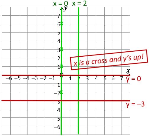
If you plot the coordinate pairs (0, 1), (0, 3), (0, 6) and (0, –2) on a coordinate grid, you’ll find that they all lie on the y-axis – in fact every point on the y-axis, including the points where the y-coordinate isn’t a whole number, has an x-coordinate of zero. So x = 0 is the equation of the vertical line that sits on the y axis.

Similarly, x = 2 is the equation of a vertical line where every point on the line has an x-coordinate of 2.

If you plot several points with a y-coordinate of zero – e.g. (2, 0), (5, 0), (-3, 0) and join them up, you get a horizontal line; this is the line y = 0, and is in the same place as the x-axis.

Do the same for y = -3 and you’ll get another horizontal line.

You might like to follow the above instructions before scrolling down to see the lines you should end up with.

Don’t forget to always use a ruler for when you are plotting a straight line graph, and label each line with its equation!

So the line x = k (where k is any constant) is always vertical, and the line y = k is always horizontal.

Other straight line graphs

Simple diagonal lines

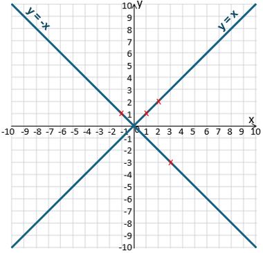
Let’s start with the simplest diagonal line: y = x.

If y is the same as x then
When x = 1, y = 1 … so the point (1, 1) will be on the line.
When x = 2, y = 2 … so (2, 2) is on the line.
Plot these two points and a few more where the x- and y-coordinates are both the same. Join them up to make a straight line graph; what does it look like?

You should get a diagonal line going from bottom left to top right, through the origin.

Now try y = -x.

When x = 3, what will y be?
Answer: y = -3 … so (3, -3) is on the line.

What about when x = -1?
y = -(-1), which of course is just 1 … so you can plot the point (-1, 1).

Do a few more and join them up to see what your line looks like.

The image below shows what you should end up with.

Changing the y-intercept and the gradient

With most straight line graphs you’ll want to draw a table of values to work out your coordinate pairs. We’ll fill it in manually in this tutorial but once you get the hang of it, or for more complex calculations, the Table function on your calculator will often make this a lot quicker. And in an exam you’ll usually be given a couple of the y-coordinates so you can just check that those ones match what the calculator is giving you, then you know you’ve entered it correctly.

Let’s plot the straight line graph of y = x + 3.

Draw out a table with the x-values you want to plot the graph for. In this example let’s just use 0 to 5:

Now, when x = 0, y will be x + 3 which is 0 + 3 = 3, so fill that in in the table.
When x = 1, y = 1 + 3 = 4
…and so on. Fill in the rest of the table and it should look like this:

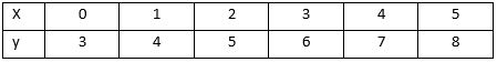
So the points we need to plot are (0, 3), (1, 4), (2, 5) and so on.

Now plot the points on a new coordinate grid, join them up to draw your straight line graph, and label it with its equation. (If you’ve only been asked to plot the graph for values of x from 0 to 5 then you don’t need to extend it beyond the plotted points, but in fact the line y = x + 3 goes on forever in both directions.)

Now let’s do the same for the line y = 2x. Start with the same blank table as before, but this time, instead of adding 3 to each value, we’re multiplying them all by 2.

Here’s what your completed table should look like:

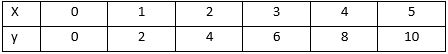
So the points to plot are (0, 0), (1, 2), (2, 4) and so on. Plot them (you can use the same coordinate grid), draw the straight line graph and label it.

Here’s what you should end up with:

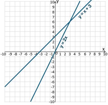
Look at how these two graphs compare with your graph of y = x from earlier.

y = x + 3 moves the whole line up by 3 units, while keeping the steepness – or gradient – the same. The y-intercept – the place where the graph crosses the y-axis – has moved up from 0 to 3. (This is a translation with vector $\begin{pmatrix}0\\3\end{pmatrix}$ : the shape doesn’t change but the whole thing moves up by 3 units.)

y = 2x still goes through the origin but is steeper than y = x.
y = x goes up by 1 unit for every 1 to the right, which means it has a gradient of 1.
y = 2x goes up 2 for every 1 to the right, which means it has a gradient of 2.

If a line goes UP from left to right then it has a positive gradient.
If it goes DOWN then the gradient is negative.
And of course if it’s horizontal then the gradient is zero.

Your turn 1

Can you predict what these straight line graphs will look like? Draw a table of values and plot the graph for each one. What is (a) its y-intercept, and (b) its gradient?

y = x + 5
y = 3x
y = x – 4
y = -2x

Click here for the answers

Varying both the y-intercept and the gradient

Now we’re going to plot the graph of y = 2x – 1.

Looking back at the graphs you’ve already done, can you predict what the y-intercept and gradient of this graph will be?

Let’s use a different range of x-values this time, so you get a bit of practice at working with negative x-values. We’ll do from -2 up to 3.

Fill in the table and plot the graph. Were your predictions correct?

Here’s what you should have got:

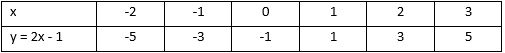
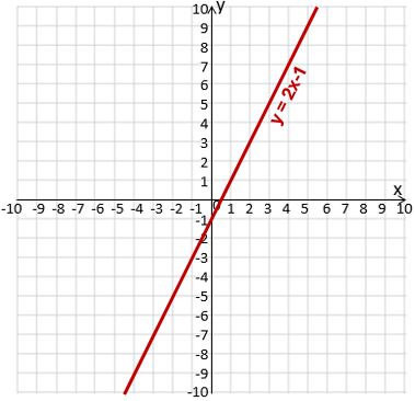
y-intercept -1, gradient 2

Your turn 2

Consider the graph of y = ½ x + 4.
a) Try to predict the y-intercept and the gradient.
b) Draw a table of values (you will get some values that aren’t whole numbers) and plot the graph for x-values from -2 to 3. Were your predictions correct?
Now do the same for the graph of y = 3 – 2x. (It might help if you think of it as y = -2x + 3.)

Click here for the answers

The general equation of a straight line, y = mx + c

Hopefully you’ve started to spot a pattern in the graphs you’ve plotted in this tutorial.

If the equation of a straight line is given in the form y = mx + c then

The c (the number on its own) is the y-intercept, i.e. the number on the y-axis where the graph crosses it.
This is also the value of y when x is 0, since any graph crosses the y-axis when x = 0 (and vice versa).
The m (the number multiplied by the x) is the gradient, i.e. how many units the graph goes up by, for each unit to the right.

If you have these two pieces of information then you can plot a graph without always having to make a table of values and plot all the points.

Your turn 3

What are the gradients and y-intercepts of these graphs? You might find it helpful to rearrange some of them so that they look more like y = mx + c.

y = 3x – 2
y = ⅔ x + 5
y = 4 + x
y = 5 – 2x

Click here for the answers

That covers the basics of straight line graphs, and takes you up to roughly GCSE Grade 3/4 level. I’ll cover more of what you need to know for the GCSE in a later tutorial.

If you’ve found this article helpful then please share it with anyone else who you think would benefit (use the social sharing buttons if you like). If you have any suggestions for improvement or other topics that you’d like to see covered, then please comment below or drop me a line using my contact form.

On my sister site at at mathscourses.co.uk you can find – among other things – a great-value suite of courses covering the entire GCSE (and Edexcel IGCSE) Foundation content, and the “Flying Start to A-level Maths” course for those who want to get top grades at GCSE and hit the ground running at A-level – please take a look!

If you’d like to be kept up to date with my new content then please sign up to my mailing list using the form at the bottom of this page, which will also give you access to my collection of free downloads.

Your turn 1 – answers

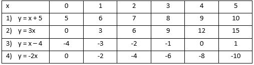
y-intercept 5, gradient 1
y-intercept 0, gradient 3
y-intercept -4, gradient 1
y-intercept 0, gradient -2 (goes DOWN 2 for every 1 to the right)

Click here to return to questions

Your turn 2 – answers

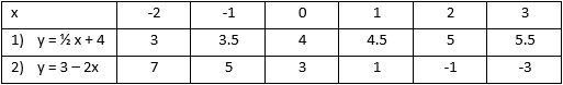
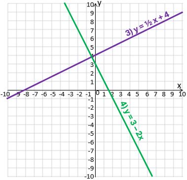
y-intercept 4, gradient ½ (goes up by ½ for every 1 to the right)
y-intercept 3, gradient -2 (goes down by 2 for every 1 to the right)

Click here to return to questions