This is part 3 of a series covering the mathematical notation you need for A-level Maths. Click the links below for the previous parts:
Part 1: set notation and miscellaneous symbols
Part 2: other Pure Maths notation

This final instalment covers vectors and the mathematical notation used for Statistics and Mechanics.

You can find an exhaustive list in the appendices to the specification published by your exam board – Edexcel (9MA0), AQA (7357), OCR (H240) and OCR/MEI (H640) – but here you’ll find a little more explanation for the ones that you’re most likely to come across.

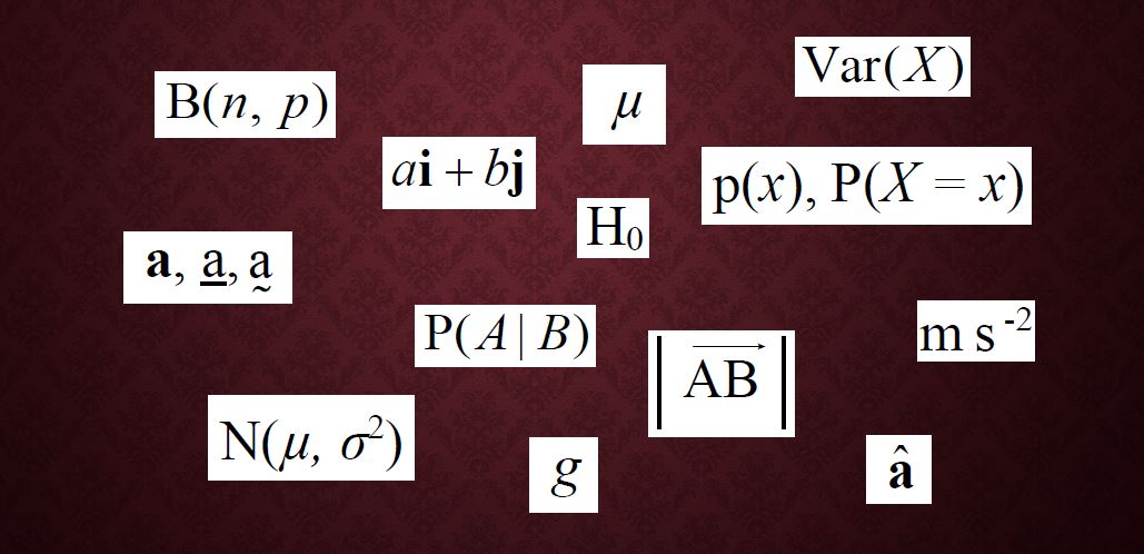
The images used here are taken from the Edexcel spec, but the list is the same for all.

Vectors

You’re probably already familiar with the majority of the mathematical notation here from GCSE, but there will be a few items you’re unlikely to have encountered before.

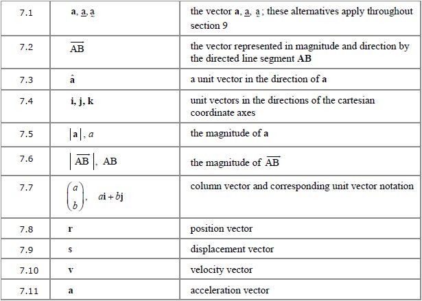
Note: in 7.2 and 7.6, the line above the AB is actually an arrow pointing to the right; it just hasn’t reproduced well here.

7.1 to 7.2 Describing vectors

Remember, when a lowercase letter is used to represent a vector, it should be in bold text if typed, or underlined (with either a squiggly or a straight line) if handwritten.

$\overrightarrow{AB}$ represents the vector from point A to point B. If the arrow is reversed then you have the vector from B to A: $\overleftarrow{AB}$ or $\overrightarrow{BA}$ .

7.3 Unit vector

The circumflex (^) above the vector indicates a unit vector: $\mathbf {\hat {a}}$ represents a vector in the same direction as vector $\mathbf{a}$ , but with a length of exactly one unit, so it’s vector $\mathbf{a}$ divided by its length (see magnitude, below).

7.4 and 7.7 i, j, k format

From GCSE you’ll be familiar with column vectors: $\begin{pmatrix}2\\-3\end{pmatrix}$ means 2 units in the x-direction (normally to the right) and -3 in the y-direction, i.e. 3 down. Similarly, you can have a 3-dimensional vector which also includes a movement in the z-direction – just add the z-component to the bottom of the column vector: $\begin{pmatrix}2\\-3\\1\end{pmatrix}$

$\mathbf{i}$ , $\mathbf{j}$ and $\mathbf{k}$ are the unit vectors in the x-, y- and z- directions respectively; in other words, $\mathbf{i}$ represents a movement of 1 unit in the x-direction.

So the column vector $\begin{pmatrix}2\\-3\end{pmatrix}$ can alternatively be written as $2\mathbf{i} - 3\mathbf{j}$ .

Similarly, $\begin{pmatrix}2\\-3\\1\end{pmatrix}$ can be written as $2\mathbf{i} - 3\mathbf{j} +\mathbf{k}$ .

You’ll often find that vectors are given in $\mathbf{i}$ , $\mathbf{j}$ format in questions, but if you find it easier to work with column vectors – I do; it involves less writing, for a start! – then it’s fine to convert them into column vector form… and there’s no need to convert them back again at the end, either.

7.5, 7.6 Magnitude of a vector

As you know from earlier, enclosing something in vertical lines denotes the modulus, or magnitude, of whatever it encloses; in this case it’s the size (length) of a vector, regardless of its direction. Essentially the modulus signs cancel out the arrow, bold text or underlining, so you also have the alternative of simply omitting both, so $|\overrightarrow{AB}| = AB$ and $|\mathbf{a}| = a$ .

For a 2-dimensional vector, the two components form the two shorter sides of a right-angled triangle, with the resultant vector being the hypotenuse, so you can find its magnitude using Pythagoras.

For example, if $\overrightarrow{AB} = \begin{pmatrix}4\\-3\end{pmatrix}$

then $|\overrightarrow{AB}| = AB =\sqrt{4^{2}+(-3)^{2}}=\sqrt{25} = 5$

This can also be extended to a 3-dimensional vector; it’s equivalent to finding the length of the diagonal of a cuboid.

7.8 to 7.11 Vectors in kinematics

These letters are used for vectors representing position, displacement, velocity and acceleration vectors. The position vector is the one that gives a location relative to the origin, and a displacement vector tells you where the body is in reference to some other point of reference, generally its starting position.

Statistics

You’ll already be familiar with some of the mathematical notation at the beginning of this table, but a lot of the later content will be (quite literally) Greek to you! My explanations may not make much sense to you until you study the relevant topics in more depth, but I’ll do what I can to keep them as simple as possible!

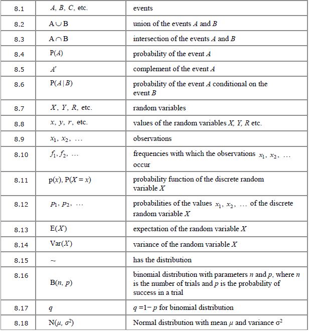
8.1 to 8.6 Set notation for probability

This is already familiar to you from the set notation section; here it’s just being used in the context of probability questions, often with Venn diagrams. The complement of event $A$ , shown as $A'$ , just means the opposite of $A$ , so $P(A')$ is the probability of event $A$ not happening.

8.7 to 8.12 Random variables

This concept is probably best explained using an example. Let’s say you have a bag with five raffle tickets numbered 6 to 10. If you draw a random ticket out of the bag then the probability of drawing, say, ticket number 7, is of course 0.2.

With the notation $P(X=x)$ , the P represents the probability of something happening, and the bit in the brackets specifies what outcome we’re looking for. Uppercase $X$ is a general description of what the variable is, in this case “the number of the ticket drawn”, and lowercase $x$ specifies which particular outcome we’re looking at the probability for – in this case ticket number 7.
So in this case, $P(X=7) = 0.2$ means “the probability that the ticket number drawn is 7, is 0.2”.

Sometimes this is abbreviated to simply $p(x)$ (with a lowercase p), so in this example $p(7) = 0.2$ .
It can then be abbreviated even further when listing the probabilites of all the possible outcomes: $p_{1}$ is the probability of outcome 1 (in this case that might mean drawing ticket no. 6, so $x_{1} = 6}$ ); $p_{2}$ is the probability of outcome 2 (ticket no. 7, $x_{2} = 7$ ), etc.

Of course, in this particular example every possible outcome has the same probability, but that won’t always be the case.

8.13, 8.14 and 8.22 to 8.27 Measures of location and spread

A measure of location is an average; at A-level the measure used most often is the mean of a distribution.

$E(X)$ is the expected, or mean, value of a discrete probability distribution. $\overline{x}$ is used for the mean calculated from a sample, and $\mu$ (Greek lowercase mu) is used for the mean of whole population.

A measure of spread tells you how spread out the data in the distribution is. The measure of spread that corresponds to the mean is the standard deviation , which can be described a “a typical distance from the mean”. Of course it depends on the shape of the distribution, but generally, the probability of an observed outcome being within one standard deviation of the mean is about two-thirds.

Finding the standard deviation involves squaring the differences between the observed values and the mean (so that they don’t simply cancel out when added up). Of course this means that, to get a measurement with the right units, we need to take the square root after processing the numbers, and the number that we take the square root of to get the standard deviation is called the variance.

We use $s$ for the standard deviation of a sample and $\sigma$ for the population standard deviation, so of course $s^{2}$ and $\sigma^{2}$ are the corresponding variances.

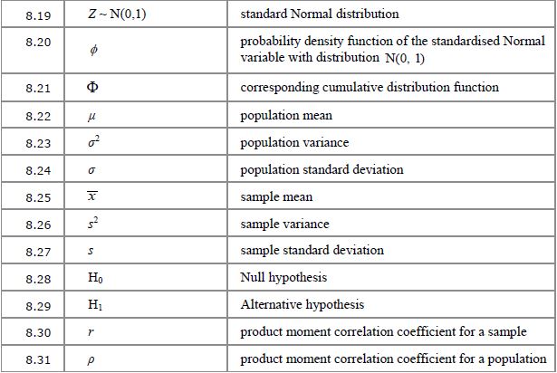
8.15 to 8.19 Probability distributions

As well as discrete probability distributions where you can write down the probability for every possible outcome (without it being too onerous), you’ll learn about binomial distributions (where you’re counting the number of “successes” out of a fixed number of trials) and normal distributions (commonly encountered with continuous data).

The definition $X \sim B(30, 0.4)$ means “the random variable X is binomially distributed with 30 trials and a probability of success in any one trial of 0.4”. For example X might the number of games of pool won by Sid if he plays 30 games and his chance of winning each game is always 0.4. You can work out the probability of him winning, for example, exactly 8 games ( $P(X = 8) = ...$ ) or at least 10 games ( $P(X \geq 10) = ...$ ).

For a normal distribution we might say $Y \sim N(150, 25)$ or “the random variable Y is normally distributed with a mean of 150 and a variance of 25” (so the standard deviation is 5). Because we’re dealing with a continuous variable, the probability is given by the area under the probability density curve. The area under a point (a single value) is 0 so you can only find probabilities for ranges of values.

8.28 and 8.29 Hypothesis testing

Hypothesis testing is a way of deciding whether something that looks as if it might have changed, actually probably has changed, based on the observation of a single sample. $H_{0}$ is the null hypothesis, the assertion that nothing has changed; $H_{1}$ is the alternative hypothesis, which proposes that there has been a change. Essentially you work out the probability of the observed result actually happening if nothing has changed, and if it turns out to be very unlikely then you reject $H_{0}$ and accept that there probably has been a change.

8.30 and 8.31 Correlation coefficients

Remember the scatter graphs you did at GCSE, where you talked about strong and weak positive and negative correlations? The product moment correlation coefficient, $r$ for a sample or $\rho$ (Greek lowercase rho) for the entire population, is a measure of how strong the correlation actually is. It ranges from 1 (perfect positive correlation with all points exactly on the line) down to -1 (perfect negative correlation).

Mechanics

There probably isn’t very much here that’s new to you.

Note, in 9.4 and 9.5, that we use negative powers in units more at A-level than you did at GCSE, but either form is acceptable.

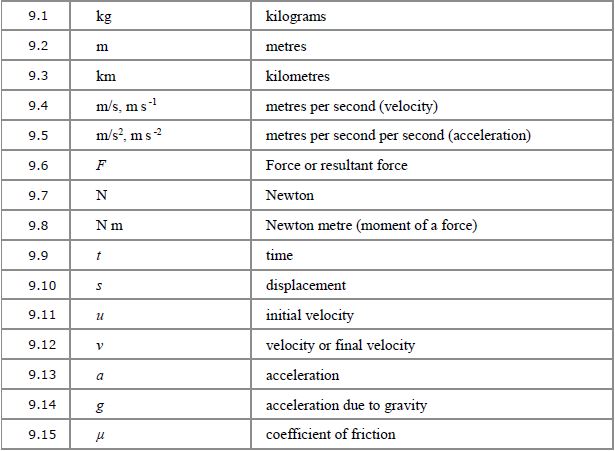
9.8 Moments

You’ll cover these in Year 2 of the A-level. A moment is the turning effect of a force and is given by force × perpendicular distance from the pivot. The units are therefore newtons × metres.

9.9 to 9.14 Constant acceleration (suvat) equations

When acceleration is constant, there’s a set of equations that you can use for kinematics calculations. $s$ is used to denote displacement (or distance), $u$ and $v$ are initial and final velocities respectively, and of course $t$ is time. $a$ is used for acceleration, but if the body is accelerating under gravity then the $a$ is replaced by $g$ , which is usually – but not always – taken to be 9.8 $ms^{-2}$ .

9.15 Friction

This is another 2nd year topic. For any two surfaces in contact, there is a coefficient of friction, $\mu$ , which is between 0 and 1 and depends on how easily the two surfaces slide across each other. The less easily they slide, the higher the value of $\mu$ .

That covers the full set of notation given in the specification.

If you’ve found this article helpful then please share it with anyone else who you think would benefit (use the social sharing buttons if you like). If you have any suggestions for improvement or other topics that you’d like to see covered, then please comment below or drop me a line using my contact form.

On my sister site at at mathscourses.co.uk you can find – among other things – a great-value suite of courses covering the entire GCSE (and Edexcel IGCSE) Foundation content, and the “Flying Start to A-level Maths” course for those who want to get top grades at GCSE and hit the ground running at A-level – please take a look!

If you’d like to be kept up to date with my new content then please sign up to my mailing list using the form at the bottom of this page, which will also give you access to my collection of free downloads.

Please share this if you find it helpful!

Mathematical notation you need for A-level – part 3