Hypothesis testing for Normal (A-level Maths)

This is part 2 of my series of three articles on hypothesis testing for A-level Maths. The first part can be found here; it gives an introduction to the concept of hypothesis testing and covers the Year 1 topic of hypothesis testing for Binomial. Part 3 (hypothesis testing for pmcc) can be found here.

This tutorial is on hypothesis testing for Normal: to decide whether the mean of a normal distribution has changed. You will need to already be familiar with the Normal distribution and how to use it to carry out probability calculations, before this article will make sense to you.

Part 3 (to follow) shows you how to ascertain whether correlation exists in a population.

Hypothesis test for the mean of a Normal population

The purpose of hypothesis testing

A hypothesis test of the mean of a normal distribution is a test to decide whether there is statistically significant evidence that the mean has changed from a known previous value. This test is for a population that is Normally distributed and has known variance σ².

For example, adjustments might have been made to a machine packing sugar into bags, and the operator wants to know whether this has increased the mean amount being packed.

How it works – basic principle

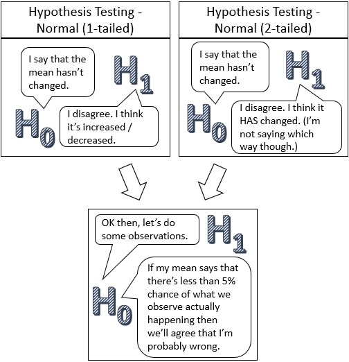
H₀ is the null hypothesis, which is the assertion that the population mean hasn’t changed from its historical value.
In the example above, the historical mean is probably just over the amount advertised on the packaging (since a certain proportion of bags sold have to be over the advertised amount), so for a 1kg bag of sugar the mean is perhaps around 1010g.

(With a mean of 1010g, if the standard deviation were – for example – 5g then the nominal 1000g content would be 2 standard deviations below the mean, so with your knowledge of the Normal distribution you should be able to work out that that would mean only 2.3% of bags would be below 1000g. With a standard deviation of 10g, 15.9% of bags would be below the 1000g threshold.)

H₁ is the alternative hypothesis, which is the assertion that the mean has changed. If the direction of change is specified then it’s a 1-tailed test; if not – effectively H₁ is sitting on the fence and not committing either way – then it’s a 2-tailed test.

We take the mean of a sample of known size and work out what the probability of that (or a more extreme) result would be if the population mean hadn’t changed.

If it’s sufficiently unlikely then we reject H₀ and accept that there probably has been a change.

Note: Because it’s all based on a balance of probabilities, you can never make a definitive statement that yes, the value in question HAS changed, only that it’s likely that it’s no longer the same as before. Therefore the question is always whether we reject H₀, not whether we accept H₁.

Distribution of sample means

Because we are using the mean of a sample, rather than just an individual item, to make our judgment, we have to use a different value from usual for the standard deviation.

Imagine you take a large number of samples from a population, with n items in each sample, and find the mean (“x-bar”) of each sample, then plot a bar chart of the sample means. The larger the sample size, the more this bar chart will resemble the bell curve for a Normal Distribution – regardless of whether the original population was Normally distributed. (If the original population was Normally distributed then the distribution of sample means will be normal regardless of the sample size.)

If the whole population has a mean of μ and a standard deviation of σ then the distribution of sample means, , has a mean of μ and a standard deviation of  (sometimes called the standard error of the mean).

Therefore the standardisation formula   becomes

Note the use of x-bar throughout (the bars aren’t showing up very well in my browser but I don’t have a way to fix that).

So for any question that mentions sample means, you should use for the standard deviation (or for the variance).

The significance level

The significance level, α, dictates how demanding the test is. If the significance level is 10%, or α = 0.1, then we’re looking to see whether the probability of the observed result (under the old mean) is less than 0.1. If it is then the result is considered significant and we reject H₀.

If α is 5%, or 0.05, then the probability has to be less than 0.05 for H₀ to be rejected – so you’re less likely to reject H₀ and to agree that the probability has most likely changed.

The significance level is also the probability of incorrectly rejecting H₀. This is because although the observed result may be unlikely, it is still possible under the old probability. At a 5% level of significance, 5% of results would be in the critical region, so it may still be a genuine result under the old probability, just one at the outer edges of what’s normally observed.

Hypothesis testing for Normal: Two possible methods

There are two possible approaches to the hypothesis test for Normal:

• With the p-value method, you find the probability (based on the old mean) of your observed result actually happening, and compare it with the significance level.
• With the test statistic /critical value method, you work out how many standard deviations above or below the old mean your observed sample mean is (this z-value is the test statistic), and how many standard deviations away you need to be for the result to be significant (the critical value), and compare the two.

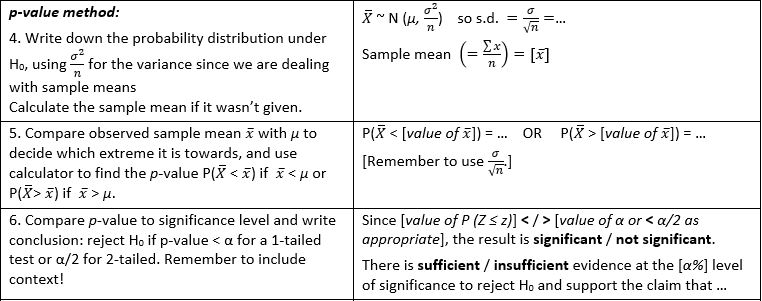
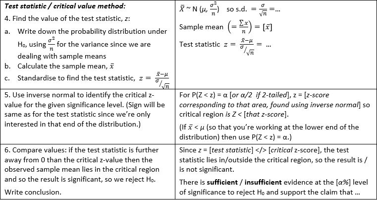
The first few steps are the same for both, but then they diverge, as shown in the writing frame below. (Scroll down for a plain text version.) You can get a free printable copy – as well as other useful downloads – if you sign up to my mailing list – see this page.

In most cases, either method is acceptable, so the p-value method is probably easier – but it’s possible that you might be asked to use the “test statistic” or “critical value(s)”, in which case you’ll need to be familiar with the second method.

A slightly simpler version of the critical value method is to find the critical value for  using the distribution of sample means, i.e. use the Inverse Normal to find the value of  for which = α [or α/2 if 2-tailed], then compare the observed value of  with the critical value and see which is further from the original mean.

Writing frame (plain text version: p-value method)

1. Define population parameter μ in context
2. Write down the null and alternative hypotheses.
3. State the significance level α.
4. Write down the probability distribution under H₀, using since we are dealing with sample means. Calculate the sample mean if it wasn’t given.
5. Compare observed sample mean  with μ to decide which extreme it is towards, and use calculator to find the p-value if , or if .
   Remember to use .
6. Compare p-value to significance level and write conclusion: reject H₀ if p-value < α for a 1-tailed test or α/2 for 2-tailed. Remember to include context!
   • Since [value of ] < / > [value of α or < α/2 as appropriate], the result is significant / not significant. There is sufficient / insufficient evidence at the [α%] level of significance to reject H₀ and support the claim that …

Writing frame (plain text version: test statistic / critical value method)

1. Define population parameter μ in context
2. Write down the null and alternative hypotheses.
3. State the significance level α.
4. Find the value of the test statistic, x:
   • Write down the probability distribution under H₀, using since we are dealing with sample means.
   • Calculate the sample mean, , if it wasn’t given.
   • Standardise to find the test statistic,
5. Use inverse normal to identify the critical z-value for the given significance level. (Sign will be same as for the test statistic since we’re only interested in that end of the distribution.)
6. Compare values: if the test statistic is further away from 0 than the critical z-value then the observed sample mean lies in the critical region and so the result is significant, so we reject H₀. Write conclusion.
   • Since z = [test statistic] </> [critical z-score], the test statistic lies in/outside the critical region, so the result is / is not significant. There is sufficient / insufficient evidence at the [α%] level of significance to reject H₀ and support the claim that …

Example of a 1-tailed test

Example

A drinks machine formerly distributed drinks of volume X ~ N (180, 16). After an overhaul, a random sample of 20 drinks is measured and the sample mean is found to be 178ml. Does this data provide evidence at the 5% level of significance that the machine is dispensing a mean volume that is less than 180ml?

Solution

(The model solution below uses the writing frame above.)

Let μ be the mean volume dispensed across all operations by the machine.
H₀: μ = 180
H₁: μ < 180           [This is a 1-tailed test since the direction is specified]
Significance level α = 0.05

p-value method:

The distribution of sample means under H₀ is  ~ N (180, )
so we use for the standard deviation.

Observed sample mean = 178
In this case < μ so we’re working at the lower end of the distribution.

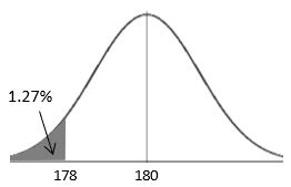
Using the distribution described above, = 0.0127

Since 0.0127 < 0.05 (i.e. a probability of 0.0127 is lower than the threshold probability of 0.05), the result is significant.
Conclusion: There is sufficient evidence at the 5% level of significance to reject H₀ and support the claim that the machine is now dispensing a mean volume less than 180ml.

Critical region method:

The distribution of sample means under H₀ is  ~ N (180, )
so we use for the standard deviation.

Observed sample mean = 178
In this case < μ so we’re working at the lower end of the distribution.

Test statistic
(i.e. our observed sample mean is 2.2361 standard deviations below the original population mean)

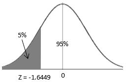
For P(Z < z) = 0.05, Z = –1.6449
(This is the boundary of critical region, i.e. the bottom 5% of the distribution of sample means goes up to 1.6449 standard deviations below the original population mean. The sample mean that we’ve actually observed is 2.2361 standard deviations below the mean so it’s in that bottom 5% of the bell curve.)

Since the test statistic z = –2.2361 < –1.6449, the test statistic lies in the critical region, so the result is significant.
Conclusion: There is sufficient evidence at the 5% level of significance to reject H₀ and support the claim that the machine is now dispensing a mean volume less than 180ml.

Alternative critical region method:

Rather than use z-scores, we can simply find the critical value of below which 5% of the distribution lies (assuming that the mean hasn’t changed).

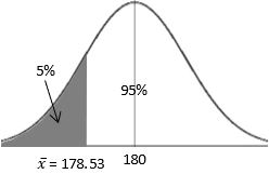
Use Inverse Normal with area (left tail) = 0.05, μ = 180 and σ = 0.89443, to obtain a critical value of 178.53 ml,
i.e.

Since 178 < 178.53 (i.e. the observed sample mean is further away from the (old) mean than the critical value is), the test statistic lies in the critical region, so the result is significant.
Conclusion: There is sufficient evidence at the 5% level of significance to reject H₀ and support the claim that the machine is now dispensing a mean volume less than 180ml.

In other words

If the mean hasn’t changed from its previous value of 180 then the probability of a random sample of 20 drinks having a mean volume of 178 ml or less, is less than 5%, so it’s likely that the mean has changed.

However, we mustn’t forget that the significance level of 5% means there’s a 5% probability that the decision to reject H₀ was wrong!

2-tailed test

If the question had asked whether the evidence suggested that the new mean volume was not equal to 180ml then a 2-tailed test would be required, so you would use α/2 = 0.025.

In the critical region method, this would mean that the critical value would be the z-score below which only 2.5% of the distribution would lie.

In fact, in this particular case the probability of the observed sample mean was still less than the 2.5% threshold, so we’d still have rejected H₀.

Your turn

The mean time taken by Parkrun participants at a particular location is historically 30.3 minutes, with a variance of 64 minutes, and may be assumed to be normally distributed. After a change is made to the route, a random sample of 400 runners is found to have a mean time of 30.9 minutes. Does this data provide evidence at the 5% significance level that the mean time for the course has changed?

Work through the writing frame, using the example solution above as a model, then check your answers by clicking on the link below.

Click here for the solution

More practice questions

1. The weight, in grams, of apples from a tree follows the distribution N (102, 49). After a new type of fertiliser is trialled, a random sample of 36 apples has a mean weight of 104g. The supplier of the fertiliser claims that the mean weight of the apples has increased. Assuming that the variance remains unchanged, test this claim at (a) the 5% level; (b) the 1% level.

2. The waiting time at a doctor’s surgery, in minutes, may be assumed to be normally distributed with mean 18 and variance 16. After a new booking system is brought in, the practice manager suggests that the mean waiting time has been reduced. A random sample of 60 patients gives a mean waiting time of 17.0 minutes. Test the claim at the 5% significance level.

3. The mean exam mark achieved on a particular paper in one year (as a percentage) follows the distribution N (57, 15²). The following year, a random sample of 100 candidates achieves a mean of 60%. Test, at the 5% significance level, the claim that the mean mark has changed.

Click here for the answers

That covers hypothesis testing for the mean of a Normal distribution. There’s one more type of hypothesis testing to cover for A-level Maths, and that’s to establish whether correlation exists in a population, and that instalment can be found here.

---

Answers:

Your turn

Let μ be the mean time taken by all Parkrun participants.
H₀: μ = 30.3
H₁: μ ≠ 30.3   
Significance level α =0.05
This is a 2-tailed test so we use α/2 = 0.025.

The distribution of sample means under H₀ is  ~ N (30.3, )
so we use for the standard deviation.

Observed sample mean = 30.9
In this case > μ so we’re working at the upper end of the distribution.

p-value method:

Don’t forget to do a sketch!

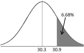
Using the distribution described above,

Since 0.0668 [p-value] > 0.05 [α], the result is not significant.
There is insufficient evidence at the 5% level of significance to reject H₀ and support the claim that the mean time for the course has changed.

Critical value method:

Test statistic
(i.e. our observed sample mean is 1.5 standard deviations above the original population mean).

Don’t forget to do a sketch!

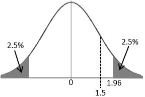
For P(Z > z) = 0.025, Z = 1.9600 (boundary of critical region, i.e. the top 2.5% of the distribution of sample means starts 1.96 standard deviations above the original population mean)

Since the test statistic z = 1.5 < 1.9600, the test statistic does not lie in the critical region, so the result is not significant.
There is insufficient evidence at the 5% level of significance to reject H₀ and support the claim that the mean time for the course has changed.

Alternative critical value method:

Using Inverse Normal with area (left tail) = 0.975 (so right tail = 0.025), μ = 30.3 and σ = 0.4,
critical value of = 31.084 mins,
i.e.

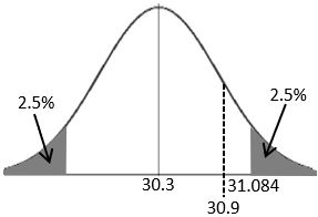
Since 30.9 < 31.084, the observed value does not lie in the critical region, so the result is not significant.
There is insufficient evidence at the 5% level of significance to reject H₀ and support the claim that the mean time for the course has changed.

Click here to return to question

More practice questions

1. p = 0.0432; z = 1.7143; (a) sufficient evidence to reject H₀        
(b) insufficient evidence to reject H₀
2. p = 0.0984; z = -1.2910; insufficient evidence to reject H₀
3. p = 0.0227; z = 2; sufficient evidence to reject H₀

Click here to return to questions