This article is part 3 of a series on the aspect of Calculus known as Differentiation; for the preceding parts see
Part 1 (introduction)
Part 2 (stationary points)
It will be relevant to you if you are studying any of:

Edexcel IGCSE Maths (though this particular section is not required for that specification)
A-level Maths
BTEC Level 3 Engineering (Module 7)

… or any other course that involves Calculus.

In part 1 we introduced the idea of differentiation and covered how to use it with simple algebraic functions and their gradients. In part 2 we looked at finding, and identifying the nature of, stationary points. In this tutorial we are going to cover increasing and decreasing functions, or intervals of increase and decrease.

What do “increasing function” and “decreasing function” mean?

Increasing or decreasing functions

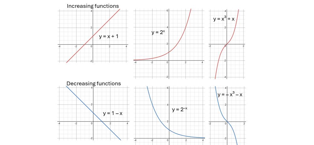
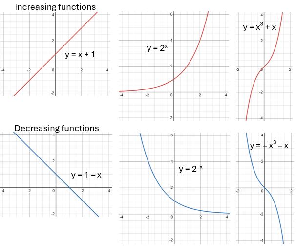
A function is increasing if, as you move from left to right across the graph, the y-coordinate is increasing…

… in other words, if the gradient is positive.

Conversely, a decreasing function is going “downhill” from left to right, i.e. it has a negative gradient.

A few examples:

Increasing and decreasing functions Increasing: y = x + 1, y = 2^x, y = x³ + x Decreasing: y = 1 - x, y = 2^(-x), y = -x³ - x

Functions that are both increasing AND decreasing

Of course, the graphs of many functions have different sections with both positive and negative gradients. For example, look at the graph of y = x², below:

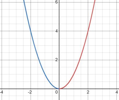
It has a negative gradient to the left of the y-axis, so it is a decreasing function for negative values of x…
and has a positive gradient to the right of the y-axis, so it is an increasing function for positive values of x.

So this is an example of a function that has an interval of decrease where x < 0, and an interval of increase where x > 0.
(And of course it has a momentary stationary point when x = 0, at which point it is neither increasing nor decreasing.)

Finding intervals of increase and decrease

To find an interval in which we have a decreasing function, we need to find the range of values of x for which $\frac{dy}{dx}< 0$ .

To find an interval of increase, we need to solve the inequality $\frac{dy}{dx} > 0$ .

For example, let’s find the interval of decrease for $y=x^2 + 6x - 7$ .

First, differentiate: $\frac{dy}{dx}=2x+6$
Then put $\frac{dy}{dx}$ less than zero and solve:
$2x+6<0$
$2x<-3$
$x<-\frac{3}{2}$

So we know that the function is decreasing when $x<-\frac{3}{2}$

To see it illustrated, you could put the original function into Desmos (opens in new tab).

Your turn 1

For each of the functions listed below, find the first derivative $\frac{dy}{dx}$ , and hence find the interval(s) of increase.

$y = 2x^2 - 8x + 5$
$y = \frac{x^3}{3} - 2x^2 - 8x$
$y = 2x^4 - x^2$
$y=\frac{2}{x}+x^2$

Click here for the answers

Demonstrating that a function is increasing (or decreasing) for all values of x

You might sometimes be asked to explain why a function is always increasing (or decreasing). To do this, you need to show that $\frac{dy}{dx}$ will always be positive (or negative).

The most likely scenario where you’ll encounter this type of question is with a cubic function. If the original function is a cubic then of course $\frac{dy}{dx}$ will be a quadratic; you then have a choice of approaches:

You can put $\frac{dy}{dx}$ into completed square form and read off the minimum value of the function (or the maximum if it’s a “sad face” curve), or
You can use the discriminant to show that the gradient curve is always above (or below) the x-axis.

Example: Demonstrate that the function $y=\frac{x^3}{3} - 2x^2 + 7x - 2$ is increasing fro all real values of x.

First, find the first derivative: $\frac{dy}{dx} = x^2 - 4x + 7$ .

In completed square form this is $(x-2)^2 + 3$ , which tells us that the minimum value of $\frac{dy}{dx}$ is 3 (and that this occurs when x = 2).
If $\frac{dy}{dx}$ can never be less than 3 then the gradient is always positive and hence the original function is increasing for all values of x.

Alternatively, using the discriminant, b² – 4ac = (-4)² – 4(1)(7) = 16 – 28 = -12.
Since b² – 4ac < 0, the curve does not cross the x-axis at any point. Since the x² term in $\frac{dy}{dx}$ is positive, the curve has a minimum point; this must be above the x-axis, so that the whole gradient curve is above the x-axis, and so the minimum gradient must be positive. Therefore the original function is increasing for all values of x.

Finding an unknown coefficient

You can also use the discriminant method to find a range of values for an unknown coefficient that will result in an increasing or decreasing function for all real values of x.

Example: Given that the function $y=\frac{x^3}{3} + kx^2 - 9x + 5$ is increasing for all real values of $x$ , find the range of possible values for $k$ .

Solution: $\frac{dy}{dx} = x^2 + 2kx + 9$
For an always-increasing gradient, we need b² – 4ac > 0 (so that the entire gradient curve is above the x-axis).
b² – 4ac = (2k)² – 4(1)(9) = 4k² – 36, < 0 => k² – 9 < 0
Critical values: (k + 3)(k – 3) = 0 => k = ±3

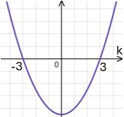
A sketch graph of y = k² – 9 shows us that the section of the graph we need is the region between the two critical values. So b² – 4ac < 0, and so the original function is increasing, when -3 < k < 3.

Your turn 2

Explain why the function $f(x) = 5 + 3x + x^2 - \frac{x^3}{3}$ is decreasing for all real values of x. Use both of the methods described above.
Given that the function $y=\frac{2}{3}x^3 + px^2 + 8x - 7$ is increasing for all real values of $x$ , find the range of possible values for $p$ .

Click here for the answers

Still to cover…

Differentiation can also be used in the context of kinematics to move between displacement, velocity and acceleration.

And it can be used to solve optimisation problems in practical situations.

I’ll cover these in future posts.

If you’ve found this article helpful then please share it with anyone else who you think would benefit (use the social sharing buttons if you like). If you have any suggestions for improvement or other topics that you’d like to see covered, then please comment below or drop me a line using my contact form.

On my sister site at at mathscourses.co.uk you can find – among other things – a great-value suite of courses covering the entire GCSE (and Edexcel IGCSE) Foundation content, and the “Flying Start to A-level Maths” course for those who want to get top grades at GCSE and hit the ground running at A-level – please take a look!

If you’d like to be kept up to date with my new content then please sign up to my mailing list using the form at the bottom of this page, which will also give you access to my collection of free downloads.

Answers:

Your turn 1 answers

$\frac{dy}{dx}=4x-8$ ; interval of increase is x > 2
$\frac{dy}{dx}=x^2 - 2x - 8$ ; intervals of increase are x < -2 and x > 4
$\frac{dy}{dx}=4x^3 - 2x = 2x(x +1)(x-1)$ ; intervals of increase are -1< x< 0 and x > 1
$\frac{dy}{dx}=-2x^{-2} + 2x$ so $-\frac{2}{x^2}+2x>0$ (can multiply through by x² without worrying about reversing the inequality since x² can never be negative); interval of increase is x > 1.

Click here to return to questions